Markov chain Monte Carlo

The sum \(Z=\sum_x e^{-E(x)/T}\) over all sets of loops is far too large to compute, and so is any average over the Boltzmann distribution. Markov chain Monte Carlo (MCMC) avoids it: it produces a long random sequence of states whose frequencies approach the Boltzmann probabilities, and averages are taken along the sequence. This page explains why that works and how to tell whether it worked.

Stochastic process and Markov chain

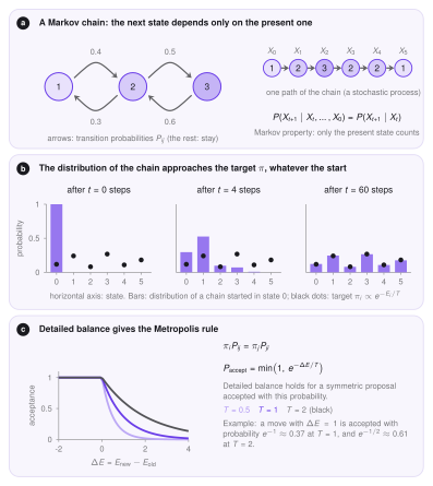
A stochastic process is a sequence of random states \(X_0,X_1,X_2,\dots\), one per time step. In general each state could depend on the whole past. A Markov chain is a process with a short memory: the next state depends only on the present one,

\[ P(X_{t+1}\mid X_t,X_{t-1},\dots,X_0)=P(X_{t+1}\mid X_t). \]

The chain is described by its transition probabilities \(P_{ij}=P(X_{t+1}=j\mid X_t=i)\). In LoopSage a state is the whole set of loops, and a step is one attempted move (slide, rebind or an epigenetic change). The past matters only through the current loops, which is what makes the chain Markov. The samples are nevertheless correlated, because consecutive states differ by one move; this is the subject of the autocorrelation section.

Which distribution does the chain reach?

A stationary distribution \(\pi\) is one that does not change under a step: if \(X_t\sim\pi\) then \(X_{t+1}\sim\pi\). The initial distribution is the distribution of \(X_0\): in LoopSage, a random start with loops placed at random. We want a chain whose stationary distribution is the Boltzmann law \(\pi_i\propto e^{-E_i/T}\) and which forgets its start.

Detailed balance is a convenient way to guarantee the first part. If \(\pi_iP_{ij}=\pi_jP_{ji}\) for every pair, then \(\pi\) is stationary. The Metropolis rule does this: propose a move to \(j\) with a symmetric proposal and accept it with probability

\[ \min\!\big(1,\,\pi_j/\pi_i\big)=\min\!\big(1,\,e^{-\Delta E/T}\big),\qquad \Delta E=E_j-E_i . \]

Moves that lower the energy are always accepted, moves that raise it with a probability that falls with \(\Delta E\) and rises with \(T\). Only the difference of energies enters, so \(Z\) is never needed.

a A three-state Markov chain and its transition probabilities. b A chain started in one state approaches the target distribution (dots). c The Metropolis acceptance as a function of \(\Delta E\) for three temperatures.

Ergodicity

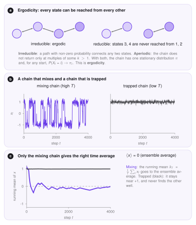
The second part, forgetting the start, is ergodicity. A chain is ergodic if it is

• irreducible: from every state there is a path with non-zero probability to every other state, so no region of states is cut off;
• aperiodic: it does not return to a state only at multiples of some period \(k>1\).

For such a chain the stationary distribution is unique, and for any start \(P(X_t=i)\to\pi_i\). In LoopSage the moves can reach any arrangement of loops (a ring can unbind and load anywhere), and the chance to stay in the same state keeps the chain aperiodic, so the chain is ergodic in principle.

In principle is not in practice. A chain can be ergodic and still trapped for a very long time. At a low temperature the sampler may stay in one valley of the energy landscape because crossing the barrier needs a move the Metropolis rule almost never accepts. This is why LoopSage uses annealing: it starts hot, where barriers are easy to cross, and cools down so that the chain settles in a deep valley.

a A chain on a connected graph is irreducible; a disconnected one is not. b A chain on a double well mixes at a high temperature and is trapped at a low one. c The running mean reaches the ensemble average only for the mixing chain.

Ergodic means

An ergodic mean is the average of a quantity \(x_t=f(X_t)\) along the chain,

\[ \bar x_T=\frac1T\sum_{t=1}^{T}x_t \;\longrightarrow\; \langle x\rangle=\sum_i \pi_i f(i)\qquad (T\to\infty). \]

The right-hand side is the ensemble average, the average over the Boltzmann distribution. The theorem says that the time average along one long ergodic chain equals it. This is what makes the whole method work: we never sum over all states, we average over snapshots.

Almost everything LoopSage reports is an ergodic mean over the snapshots after the burn-in: the contact map implied by the loops, the mean loop length, the unfolded fraction, the average of each energy term, the occupancy of each bead by a loop leg, and the insulation or stripe profiles computed from the averaged map. The averaged MD contact map is the same kind of quantity over the 3D frames. These are meaningful when the chain has converged and the number of snapshots is large compared with the correlation time.

What is not an ergodic mean: a single snapshot, the last snapshot, the minimum energy found, and any average that includes the burn-in or the annealing phase (the chain is then not stationary).

Reading a run: the burn-in

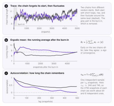
A chain that starts away from the typical states first drifts, and only later fluctuates around a constant level. The drifting part is the burn-in and is discarded. The mean loop length is a good indicator: at the start the rings are short, it rises, and in equilibrium it should stay almost constant with fluctuations. A curve that keeps rising or falling is not equilibrated.

Two real LoopSage chains (Metropolis, \(T=1\), 250 beads, 39 extruders, 200 000 steps, one snapshot per 40 steps). a The trace of the mean loop length. b The running mean after the burn-in. c The autocorrelation function. Purple is chain 1 and black chain 2.

Autocorrelation: how long the chain remembers

Consecutive snapshots are similar, so the samples are not independent. The autocorrelation function measures how similar a quantity is to itself after a delay of \(k\) snapshots (the lag),

\[ \rho(k)=\frac{\operatorname{cov}(x_t,\,x_{t+k})}{\operatorname{var}(x_t)},\qquad \rho(0)=1 . \]

How to read it. \(\rho(k)=1\) means the two values are identical, \(\rho(k)=0\) means that they are unrelated, and a negative value means that they tend to be opposite. A plot of \(\rho\) against \(k\) starts at 1 and decays. The lag at which it reaches about 0 is the time after which the chain has forgotten where it was: samples further apart than that are practically independent. A curve that stays high for hundreds of lags says that the chain moves slowly through the states.

The decay is summarised by the integrated autocorrelation time,

\[ \tau_{\mathrm{int}}=1+2\sum_{k\ge1}\rho(k), \]

the number of snapshots that are worth one independent sample. With \(T\) snapshots the effective sample size is

\[ \mathrm{ESS}=\frac{T}{\tau_{\mathrm{int}}}, \]

and the error of an ergodic mean is about \(\sigma/\sqrt{\mathrm{ESS}}\), with \(\sigma\) the standard deviation of the quantity. In the figure above \(\tau_{\mathrm{int}}\approx240\) and \(740\) snapshots, so each chain of 4750 snapshots after the burn-in is worth only about 20 and 6 independent samples of the mean loop length. This is the honest measure of how much the run knows.

In practice

Plot the trace: it should fluctuate around a constant after the burn-in. Run two chains from different random starts (replicas): their running means must agree, as in panel b. Read \(\tau_{\mathrm{int}}\) off the autocorrelation: if it is a large share of the run, increase n_steps, not only the number of snapshots (saving more often adds correlated samples, not new ones). The Monte Carlo page lists the settings, and the report shows the drift of the energy between the two halves of the run.