Mechanics of LoopSage

LoopSage assigns an energy to every set of loops and samples sets with probability \(\propto e^{-E/T}\). This page explains where that idea comes from, why it is only an approximation for a living cell, and what is kept from the exact theory. New words are defined when they appear.

The mechanical Hamiltonian

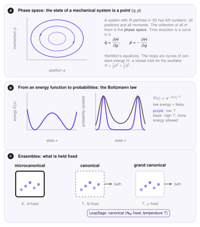
In classical mechanics a system of \(N\) particles is described by the positions \(q\) and momenta \(p\) of all particles. Together they form a point \((q,p)\) in the phase space, a space with \(6N\) coordinates (three positions and three momenta per particle). The Hamiltonian \(H(q,p)\) is the total energy as a function of this point: kinetic plus potential, for example \(H=\tfrac12p^2+\tfrac12q^2\) for an oscillator. It determines the motion through Hamilton's equations,

\[ \dot q=\frac{\partial H}{\partial p},\qquad \dot p=-\frac{\partial H}{\partial q}, \]

where a dot is the derivative with respect to time. The system moves along a curve of constant energy.

This needs \(H\) to be differentiable: the force is the derivative of the energy, so a smooth landscape gives a well-defined motion. The energy of the loop model is not like that. A loop has integer positions \((m,n)\) on a grid of beads, so there is no derivative, and the loops do not follow equations of motion. Loop extrusion in LoopSage is a statistical model, and for it only a weaker notion of Hamiltonian is kept.

a A mechanical state is a point in phase space and moves along a curve of constant energy. b An energy landscape turns into probabilities by the Boltzmann law; a higher temperature allows higher energies. c Ensembles differ by what is held fixed.

The statistical Hamiltonian

In statistical physics the Hamiltonian can be any function \(E(x)\) that gives the energy of a state \(x\), with no need for derivatives or motion. Then the probability of a state at temperature \(T\) is the Boltzmann law,

\[ P(x)=\frac{1}{Z}\,e^{-E(x)/T},\qquad Z=\sum_x e^{-E(x)/T}. \]

\(Z\) is the partition function, the number that makes the probabilities sum to one. Low-energy states are likely, and \(T\) sets how much higher energy is tolerated. In LoopSage \(T\) is in arbitrary units, because the energy itself is made of effective terms (folding, binding, crossing) and not of physical joules. A state \(x\) is the complete set of loops \(\{(m_i,n_i)\}\), possibly with the epigenetic states of the beads.

Ensembles

An ensemble is the set of all states together with their probabilities, for a given set of conditions. The three classical ones differ in what is held fixed.

Ensemble	Fixed	Exchanges with the outside
microcanonical	energy \(E\), particle number \(N\)	nothing (isolated)
canonical	temperature \(T\), particle number \(N\)	energy (a heat bath)
grand canonical	temperature \(T\), chemical potential \(\mu\)	energy and particles

LoopSage uses the canonical ensemble: the number of extruders \(N_{\mathrm{lef}}\) is fixed, and the temperature \(T\) controls the fluctuations. This is why the Boltzmann law above is the right distribution, and why the Metropolis rule on the Monte Carlo page works. The grand canonical alternative, with extruders appearing and disappearing, is mimicked by the rebinding move, where one ring is removed and another loaded.

A cell is not in equilibrium

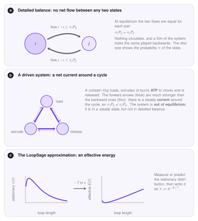
The Boltzmann law describes a system in equilibrium. A cohesin ring is not in equilibrium: it burns ATP to extrude, and it loads and unloads in a cycle. This is a driven system.

What distinguishes equilibrium is detailed balance. Let \(\pi_i\) be the probability of state \(i\) and \(P_{ij}\) the probability to jump from \(i\) to \(j\) in one step. Detailed balance says that for every pair of states the two flows are equal,

\[ \pi_i\,P_{ij}=\pi_j\,P_{ji}. \]

Nothing circulates: a film of the system looks the same played backwards. In a driven cycle (load, extrude, release) the forward flow is much larger than the backward one, so there is a steady current and detailed balance is broken. The system is then in a steady state: the probabilities \(\pi\) do not change with time, but they are not Boltzmann probabilities.

a Detailed balance: equal flows for every pair. b A driven cycle has a net current, so it is out of equilibrium. c LoopSage takes the stationary distribution and writes it as an effective energy.

The LoopSage approximation

LoopSage does not model the driving. It turns the problem around: whatever the stationary distribution \(\pi\) of the loops is, write it as

\[ \pi(x)\propto e^{-E(x)/T}. \]

The energy is then an effective energy, \(E=-T\ln\pi\) up to a constant: it is not the physical energy of the ring but a compact way of saying which loop sets are likely. The terms of \(E\) are chosen to reproduce what is observed. Long loops are favoured (folding), legs prefer CTCF sites (binding), and crossing loops are forbidden (crossing). The coefficients are fitted by the optimizer to Hi-C or to the input loops.

This is an approximation with a clear limit. Equilibrium sampling gives the right average map and the right fluctuations if the effective energy is right, but it does not give the dynamics: the sampler's steps are not real time, and currents such as the directed motion of a ring are replaced by random-walk moves. Questions about speed, residence times or the order of events need a model with real kinetics.

How detailed balance is approximated

The sampler (MCMC) is built so that it satisfies detailed balance with respect to \(e^{-E/T}\) by construction: a proposed move is accepted with the Metropolis probability, which makes \(\pi_iP_{ij}=\pi_jP_{ji}\) for the target distribution. Three choices keep this approximately true in practice.

• Symmetric proposals. Sliding by \(\pm1\) is as likely as the reverse move, so the proposal does not bias the result.
• Rebinding as an approximation. The rebinding move (load a minimal loop anywhere) is not exactly the reverse of the extrusion, so it is a loading process rather than an exactly balanced move. With uniform loading it is close to symmetric. A loading track makes it deliberately biased towards the real loading sites.
• Annealing. With method = Annealing the temperature changes during the run, so the chain is not stationary until the end. Only the snapshots after the burn-in, when the temperature is close to its final value, are used for statistics.

In LoopSage

The energy terms and the temperature are described in Monte Carlo. The next page explains why the sampler converges to the Boltzmann distribution and how to check that it did.